Intro to Excel 2010

Basic Formatting:

MS Excel 2016

American University

Office of Information Technology

Training Unit

Office of Information   Technology  Introduction to Microsoft Excel 2016 
i 
 
INTRODUCTION ..................................................................................................................................................... 1 
The Excel 2016 Environment .................................................................................................................................. 1 
Worksheet Views ................................................................................................................................................... 2 
UNDERSTANDING CELLS ................................................................................................................................... 2 
Select a Cell ........................................................................................................................................................... 3 
Select a Cell Range ................................................................................................................................................. 4 
CELL CONTENT ...................................................................................................................................................... 4 
Enter and Edit Data ................................................................................................................................................ 4 
Delet or Edit the Contents of a Cell ........................................................................................................................ 5 
Change Entries while Typing .................................................................................................................................. 5 
Copy and Paste Cell Content .................................................................................................................................. 6 
Cut and Paste Cell Content..................................................................................................................................... 6 
Access More Paste Options .................................................................................................................................... 7 
Use the Fill Handle ................................................................................................................................................. 8 
Continue a Series with the Fill Handle.................................................................................................................... 8 
Use Flash Fill .......................................................................................................................................................... 9 
FIND AND REPLACE ............................................................................................................................................. 9 
Find Content .......................................................................................................................................................... 9 
Replace Content .................................................................................................................................................. 10 
WORKING WITH ROWS, COLUMNS AND CELLS .................................................................................... 11 
Modify Column Width ......................................................................................................................................... 11 
Modify Row Height .............................................................................................................................................. 11 
Modify All Rows or Columns ................................................................................................................................ 11 
Insert Rows .......................................................................................................................................................... 12 
Insert Columns ..................................................................................................................................................... 13 
Delete Rows......................................................................................................................................................... 13 

Office of Information   Technology  Introduction to Microsoft Excel 2016 
ii 
 
Delete Columns ................................................................................................................................................... 13 
Wrap Text and Merge Cells .................................................................................................................................. 14 
Wrap Text in Cells ................................................................................................................................................ 14 
Merge Cells Using the Merge & Center Command ............................................................................................... 14 
FORMATTING A WORKSHEET ...................................................................................................................... 15 
Text Alignment .................................................................................................................................................... 15 
Change Horizontal Text Alignment....................................................................................................................... 15 
Change Vertical Text Alignment ........................................................................................................................... 15 
Cell Borders and Fill Colors .................................................................................................................................. 15 
Add a Border........................................................................................................................................................ 15 
Add a Fill Color ..................................................................................................................................................... 16 
Format Text and Numbers ................................................................................................................................... 16 
Apply Number Formatting ................................................................................................................................... 16 
WORKING WITH DATA – FREEZE PANES ................................................................................................ 17 
Freeze Rows ......................................................................................................................................................... 17 
Freeze Columns ................................................................................................................................................... 17 
USING FORMULAS AND FUNCTIONS ......................................................................................................... 18 
Order of Operations ............................................................................................................................................. 18 
Create a Formula ................................................................................................................................................. 18 
Common Functions .............................................................................................................................................. 19 
Create a Function Using the AutoSum Command ................................................................................................ 19 
RELATIVE AND ABSOLUTE CELL REFERENCES ................................................................................... 20 
Relative References ............................................................................................................................................. 20 
Absolute references ............................................................................................................................................. 20 
PASTE SPECIAL ................................................................................................................................................... 21 
RANGE NAMES .................................................................................................................................................... 22 

Office of Information   Technology  Introduction to Microsoft Excel 2016 
iii 
 
WORKING WITH DATA – SORT AND FILTER ......................................................................................... 24 
Sort a Sheet ......................................................................................................................................................... 24 
Sort a Range ........................................................................................................................................................ 24 
Autofilter ............................................................................................................................................................. 25 
Using Filter to Sort ............................................................................................................................................... 25 
PRINTING THE WORKSHEET ........................................................................................................................ 26 
Work with Headers and Footers .......................................................................................................................... 26 
Print the Active Worksheet .................................................................................................................................. 26 
Print the Entire Workbook ................................................................................................................................... 27 
Print a Selection or Set the Print Area .................................................................................................................. 27 
SAVING A FILE ..................................................................................................................................................... 28 
Save a Workbook ................................................................................................................................................. 29 
Use Save As to Make a Copy ................................................................................................................................ 29 
Export a Workbook as a PDF File ......................................................................................................................... 29 
   

Office of Information Technology Introduction to Microsoft Excel 2016

INTRODUCTION

EXCEL is an Electronic Spreadsheet Program. An e-spreadsheet is a computer software program that is

used for storing, organizing and manipulating data. Electronic spreadsheet programs were originally

based on paper spreadsheets used for accounting. As such, the basic layout of computerized

spreadsheets is the same as the paper ones. Excel allows you to perform sophisticated calculations and

create formulas to automatically calculate answers. The advantage of using formulas is that when data

in the worksheet changes, all of the formulas will automatically recalculate.

Excel can store multiple spreadsheet pages in a single computer file. The saved computer file is often

referred to as a workbook and each page in the workbook is a separate worksheet.

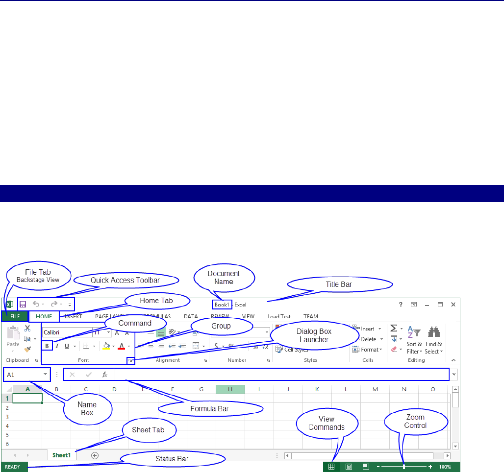
THE EXCEL 2016 ENVIRONMENT

When you open Excel 2016 for the first time, the Excel Start Screen will appear. From here, you'll be able

to create a new workbook, choose a template, or access your recently edited workbooks.

Office of Information Technology Introduction to Microsoft Excel 2016

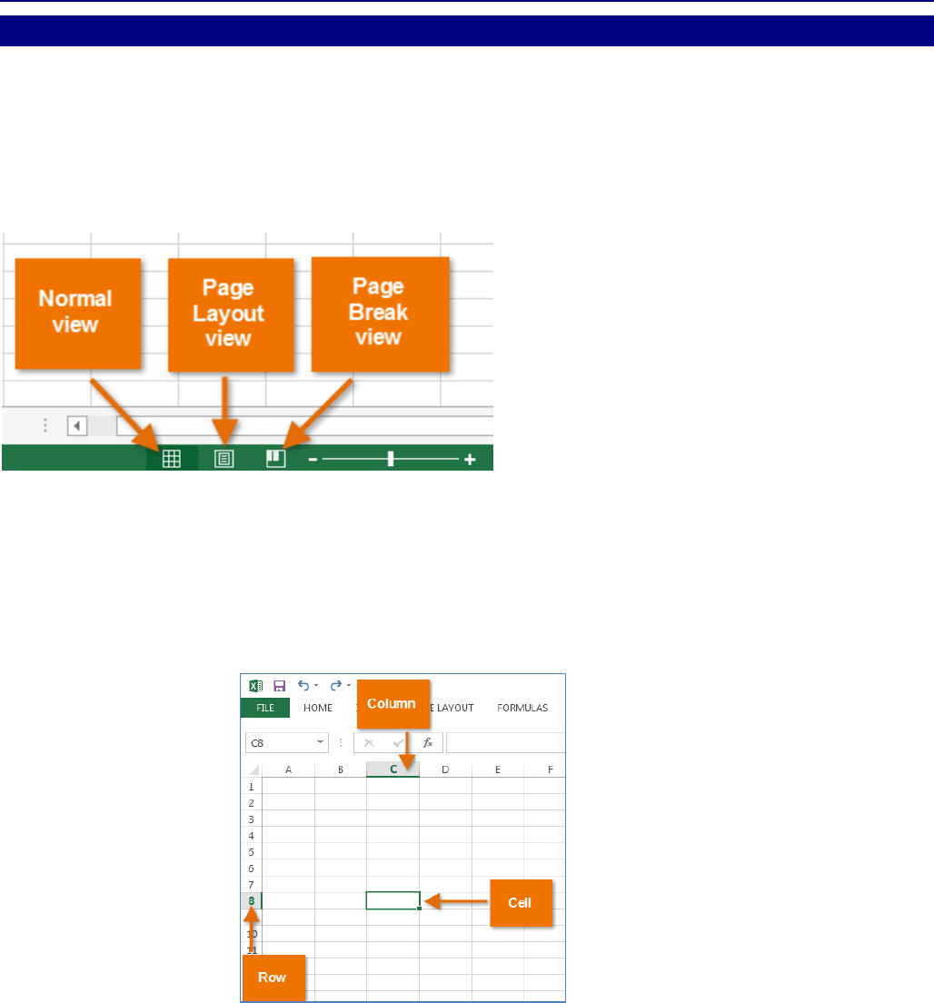
WORKSHEET VIEWS

Excel 2016 has a variety of viewing options that change how your workbook is displayed. You can choose

to view any workbook in Normal view, Page Layout view, or Page Break view. These views can be useful

for various tasks, especially if you're planning to print the spreadsheet.

1. To change worksheet views, locate and select the desired WORKSHEET VIEW command in

the bottom-right corner of the Excel window.

UNDERSTANDING CELLS

Every worksheet is made up of thousands of rectangles, which are called cells. A cell is

the intersection of a row and a column. Columns are identified by letters (A, B, C) and rows are

identified by numbers (1, 2, 3).

Office of Information Technology Introduction to Microsoft Excel 2016

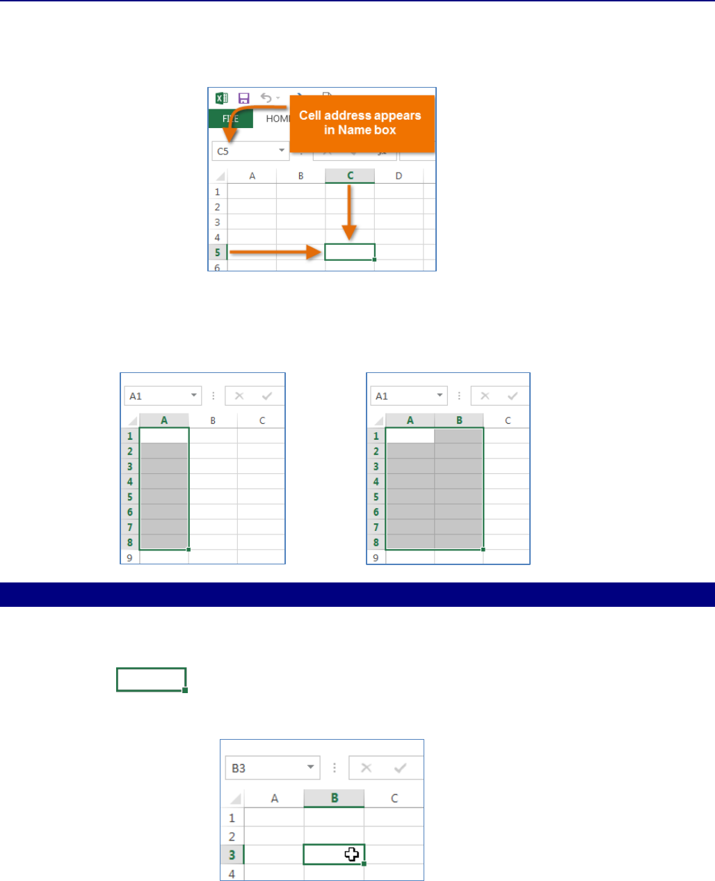
Every cell has its own name, or cell address, based on its column and row. In this example, the selected

cell intersects column C and row 5, so the cell address is C5. The cell address will also appear in

the NAME box. Note that a cell's column and row headings are highlighted when the cell is selected.

You can also select multiple cells at the same time. A group of cells is known as a cell range. Rather than

a single cell address, you will refer to a cell range using the cell addresses of the first and last cells in the

cell range, separated by a colon. For example, a cell range that included cells A1, A2, A3, A4 and A5

would be written as A1:A5.

SELECT A CELL

To input or edit cell content, you'll first need to select the cell.

1. Click a cell to select it.

2. A border will appear around the selected cell and the column heading and row

heading will be highlighted. The cell will remain selected until you click another cell in the

worksheet. You can also select cells using the arrow keys on your keyboard.

Office of Information Technology Introduction to Microsoft Excel 2016

SELECT A CELL RANGE

Sometimes you may want to select a larger group of cells, or cell range.

1. Click, hold and drag the mouse until all of the adjoining cells you wish to select are highlighted.

2. Release the mouse to select the desired cell range. The cells will remain selected until you click

another cell in the worksheet.

CELL CONTENT

Any information you enter into a spreadsheet will be stored in a cell. Each cell can contain several

different kinds of content, including text, formatting, formulas and functions.

ENTER AND EDIT DATA

1. Select the cell in which you want to display the data; use the mouse to click on a cell to select it,

or use the arrow movement keys on your keyboard to select a cell.

2. Begin typing data (numbers, text or formulas).

3. Enter the data into the cell by using any of these techniques:

a. press the [ENTER] key;

b. press any keyboard movement keys, such as the RIGHT ARROW or TAB keys;

c. or click the ENTER button in the formula bar (the boxed checkmark).

Worksheet cells can contain constant values (text or numbers) and formulas. By default, text is left-

aligned in the cell and numbers are right-aligned. Changing the alignment of the data does not change

the data type.

Office of Information Technology Introduction to Microsoft Excel 2016

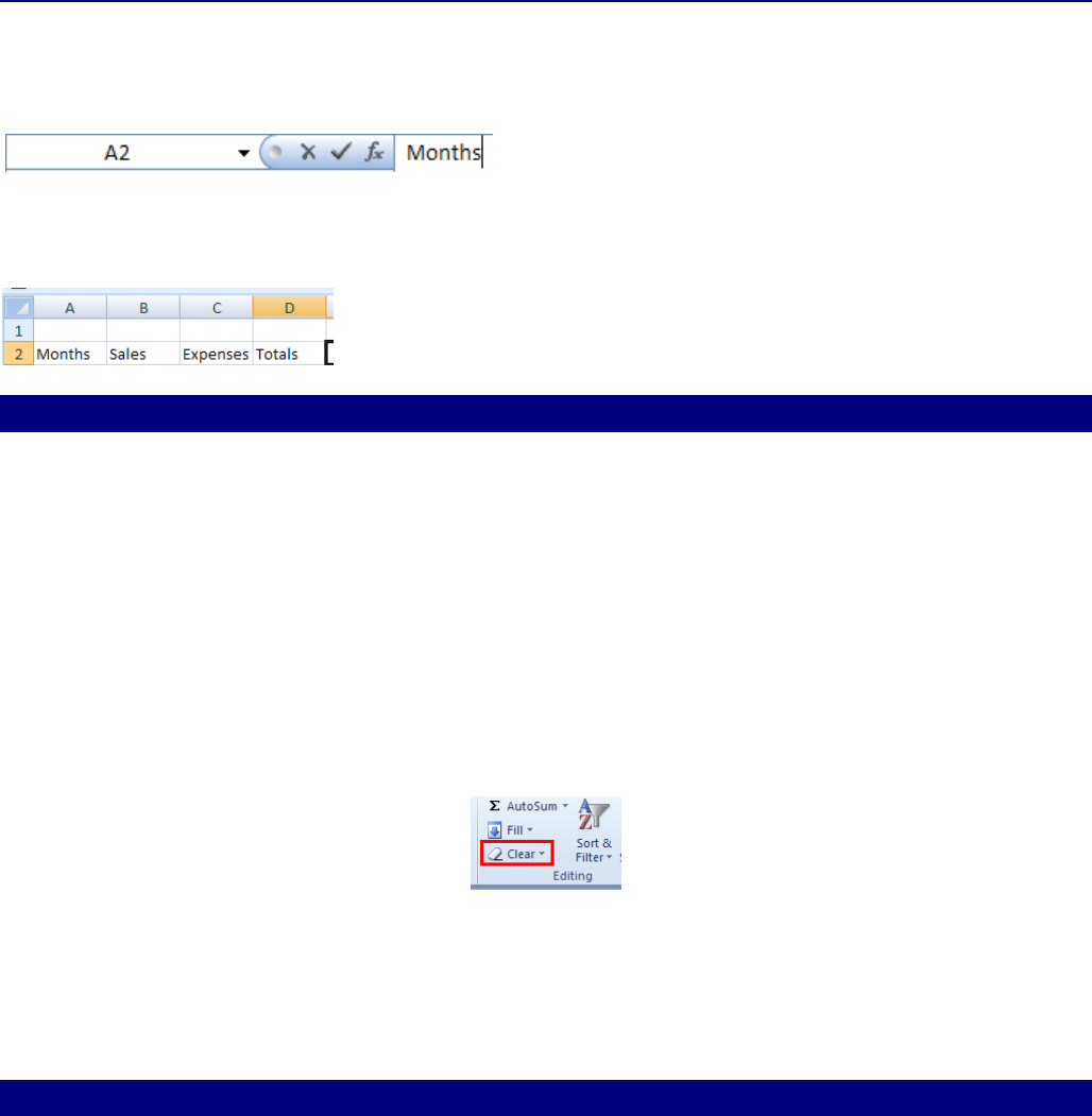
EXERCISE: ENTERING TEXT

1. Type Months and do not press the [ENTER] key.

The word appears both in the formula bar , and in the cell, but it is not yet entered.

2. Press the [ENTER] key to enter the text and move down or across one cell. The mode indicator in

the lower right of the Status Bar returns to Ready.

DELET OR EDIT THE CONTENTS OF A CELL

EDIT

1. RETYPE the entry and enter it again. The new entry replaces the old entry.

2. DOUBLE-CLICK the cell which places the cursor in the cell.

3. Press the F2 key which places the cursor in the cell at the end of the entry.

DELETE

1. Select the cell and press the [DELETE] key on your keyboard.

2. Place the cursor on the fill handle (black square in the lower-right corner of the cell, hold the left

mouse button and drag upward thru the cell.

3. Click the ERASER icon in the EDITING tab on the HOME tab.

Note:

 If you press the [DELETE] or [BACKSPACE] keys when a cell is selected, Excel removes the cell

contents but does not remove any comments or cell formats.

 If you choose CLEAR ALL from the Eraser icon, Excel removes the contents, formats, and

comments, from a cell.

CHANGE ENTRIES WHILE TYPING

To change an entry before it is entered into a cell:

1. Press the [BACKSPACE] key to delete individual characters.

2. Press the [ESC] key or click on the CANCEL button (the X in the formula bar) to clear the entire

entry.

Office of Information Technology Introduction to Microsoft Excel 2016

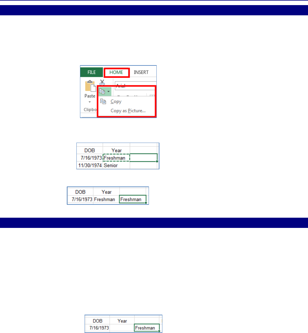
COPY AND PASTE CELL CONTENT

Excel allows you to copy content that is already entered into your spreadsheet and paste that content to

other cells, which can save you time and effort.

1. Select the cell(s) you wish to copy.

2. Click the COPY command on the HOME tab or press CTRL+C on your keyboard.

3. Select the cell(s) where you wish to paste the content. The copied cells will now have a dashed

box around them.

4. Click the PASTE command on the HOME tab, or press CTRL+V on your keyboard, or press ENTER.

CUT AND PASTE CELL CONTENT

Unlike copying and pasting, which duplicates cell content, cutting allows you to move content between

cells.

1. Select the cell(s) you wish to cut.

2. Click the CUT command on the HOME tab or press CTRL+X on your keyboard.

3. Select the cells where you wish to paste the content. The cut cells will now have a dashed

box around them.

4. Click the PASTE command on the HOME tab or press CTRL+V on your keyboard.

5. The cut content will be removed from the original cells and pasted into the selected cells.

Office of Information Technology Introduction to Microsoft Excel 2016

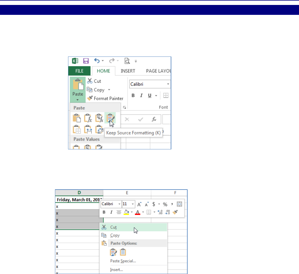
ACCESS MORE PASTE OPTIONS

You can also access additional PASTE options, which are especially convenient when working with cells

that contain formulas or formatting.

1. To access more PASTE options, click the drop-down arrow on the PASTE command.

2. Rather than choosing commands from the Ribbon, you can also access commands quickly

by right-clicking. Simply select the cell(s) you wish to format, then right-click the mouse. A drop-

down menu will appear, where you'll find several commands also located on the Ribbon.

Office of Information Technology Introduction to Microsoft Excel 2016

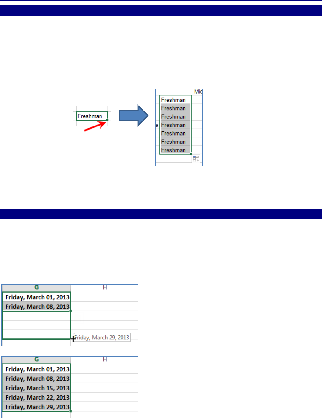
USE THE FILL HANDLE

There may be times when you need to copy the content of one cell to several other cells in your

worksheet. You could copy and paste the content into each cell, but this method would be very time

consuming. Instead, you can use the fill handle to quickly copy and paste content to adjacent cells in the

same row or column.

1. Select the cell(s) containing the content you wish to use. The fill handle will appear as a small

square in the bottom-right corner of the selected cell(s).

2. Click, hold and drag the Fill handle until all the cells you wish to fill are selected.

3. Release the mouse to fill the selected cells.

CONTINUE A SERIES WITH THE FILL HANDLE

The fill handle can also be used to continue a series. Whenever the content of a row or column follows a

sequential order, like numbers (1,2,3) or days (Monday, Tuesday, Wednesday), the fill handle can guess

what should come next in the series. In many cases, you may need to select multiple cells before using

the fill handle to help Excel determine the series order. In our example below, the Fill handle is used to

extend a series of dates in a column.

Office of Information Technology Introduction to Microsoft Excel 2016

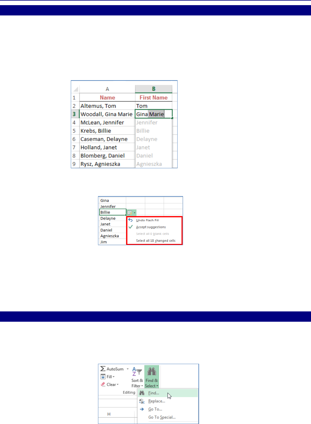
USE FLASH FILL

Flash Fill can enter data automatically into your worksheet, saving you a lot of time and effort. Just like

the Fill handle, Flash Fill can guess what kind of information you're entering into your worksheet. In the

example below, we'll use Flash Fill to create a list of first names using a list of existing full names.

1. Enter the desired information into your worksheet. A Flash Fill preview will appear below the

selected cell whenever Flash Fill is available.

 If FLASH FILL does not activate, press CTRL + E.

2. Press ENTER. The Flash Fill data will be added to the worksheet.

3. To modify or undo Flash Fill, click the Flash Fill button next to recently added Flash Fill data.

FIND AND REPLACE

When working with a lot of data in Excel, it can be difficult and time consuming to locate specific

information. You can easily search your workbook using the FIND feature, which also allows you to

modify content using the REPLACE feature.

FIND CONTENT

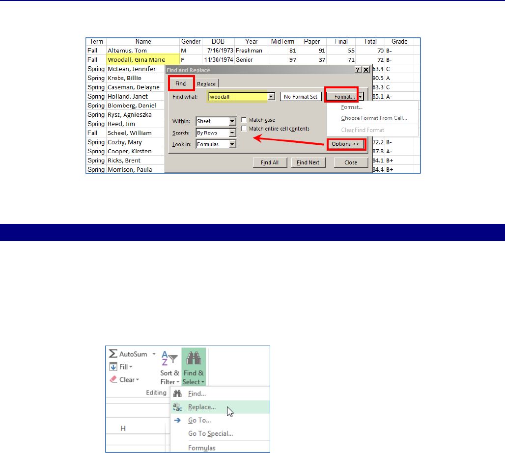
1. From the HOME tab, click the FIND AND SELECT command, then select FIND... from the drop-

down menu.

 You can also access the FIND command by pressing CTRL+F on your keyboard.

2. The Find and Replace dialog box will appear. Enter the content you wish to find.

Office of Information Technology Introduction to Microsoft Excel 2016

3. Click FIND NEXT. If the content is found, the cell containing that content will be selected.

4. Click FIND NEXT to find further instances or FIND ALL to see every instance of the search term.

5. When you are finished, click CLOSE to exit the Find and Replace dialog box.

REPLACE CONTENT

At times, you may discover that you've repeatedly made a mistake throughout your workbook (such as

misspelling someone's name), or that you need to exchange a particular word or phrase for another. You

can use Excel's Find and Replace feature to make quick revisions. In our example, we'll use Find and

Replace to correct a list of email addresses.

1. From the HOME tab, click the FIND AND SELECT command, then select REPLACE... from the

drop-down menu.

2. The Find and Replace dialog box will appear. Type the text you wish to find in the FIND

WHAT: field.

3. Type the text you wish to replace it with in the REPLACE WITH: field, then click FIND NEXT.

4. If the content is found, the cell containing that content will be selected.

5. Review the text to make sure you want to replace it.

6. If you wish to replace it, select one of the replace options:

o REPLACE will replace individual instances.

o REPLACE ALL will replace every instance of the text throughout the workbook. In our

example, we'll choose this option to save time.

7. A dialog box will appear, confirming the number of replacements made. Click OK to continue.

The selected cell content will be replaced.

8. When you are finished, click CLOSE to exit the Find and Replace dialog box.

Office of Information Technology Introduction to Microsoft Excel 2016

WORKING WITH ROWS, COLUMNS AND CELLS

By default, every row and column of a new workbook is always set to the same height and width. Excel

allows you to modify column width and row height in a variety of different ways, including wrapping

text and merging cells.

MODIFY COLUMN WIDTH

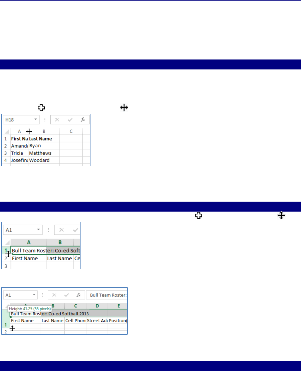
In our example below, some of the content in column A cannot be displayed. We can make all of this

content visible by changing the width of column A.

1. Position the mouse over the column line in the column heading so that the white

cross becomes a double arrow .

2. Click, hold and drag the mouse to increase or decrease the column width.

3. Release the mouse. The column width will be changed.

MODIFY ROW HEIGHT

1. Position the cursor over the row line so that the white cross becomes a double arrow .

2. Click, hold and drag the mouse to increase or decrease the row height.

3. Release the mouse. The height of the selected row will be changed.

MODIFY ALL ROWS OR COLUMNS

Rather than resizing rows and columns individually, you can also modify the height and width of every

row and column at the same time. This method allows you to set a uniform size for every row and

column in your worksheet.

Office of Information Technology Introduction to Microsoft Excel 2016

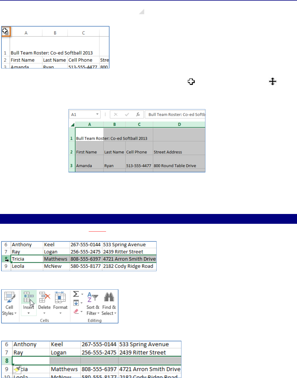
1. Locate and click the SELECT ALL button , ,just below the formula bar to select every cell in

the worksheet.

2. Position the mouse over a row line so that the white cross becomes a double arrow .

3. Click, hold and drag the mouse to increase or decrease the row height.

4. Release the mouse when you are satisfied with the new row height for the worksheet.

After you've been working with a workbook for a while, you may find that you want to insert

new columns or rows, delete certain rows or columns, move them to a different location in the

worksheet, or even hide them.

INSERT ROWS

1. Select the row heading below where you want the new row to appear. For example, if you want

to insert a row between rows 7 and 8, select row 8.

2. Click the INSERT command on the HOME tab.

3. The new row will appear above the selected row.

Office of Information Technology Introduction to Microsoft Excel 2016

INSERT COLUMNS

1. Select the column heading to the right of where you want the new column to appear. For

example, if you want to insert a column between columns D and E, select column E.

2. Click the Insert command on the Home tab.

3. The new column will appear to the left of the selected column.

NOTE: When inserting rows and columns, make sure you select the entire row or column by clicking

the heading. If you select just a cell in the row or column, the INSERT command will only insert a new

cell.

DELETE ROWS

1. Select the row(s) you want to delete.

2. Click the DELETE command on the HOME tab.

3. The selected row(s) will be deleted and the rows below will shift up.

DELETE COLUMNS

1. Select the columns(s) you want to delete.

2. Click the DELETE command on the HOME tab.

4. The selected columns(s) will be deleted and the columns to the right will shift left.

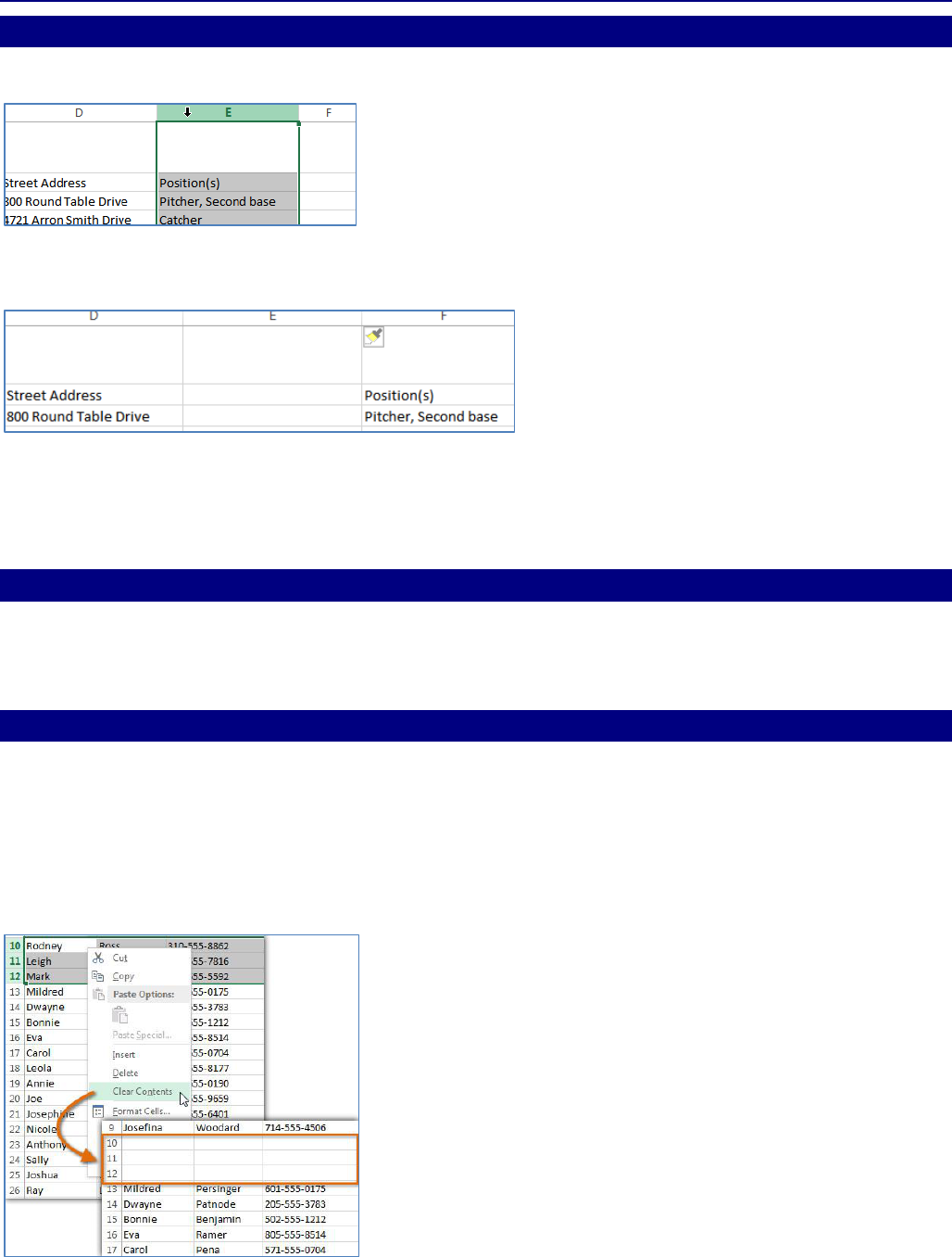
 It's important to understand the difference between deleting a row or column and

simply clearing its contents. If you want to remove the content of a row or column

without causing others to shift, right-click a heading and then select CLEAR

CONTENTS from the drop-down menu.

Office of Information Technology Introduction to Microsoft Excel 2016

WRAP TEXT AND MERGE CELLS

Whenever you have too much cell content to be displayed in a single cell, you may decide to wrap the

text or merge the cell rather than resizing a column. Wrapping the text will automatically modify a

cell's row height, allowing the cell contents to be displayed on multiple lines. Merging allows you to

combine a cell with adjacent, empty cells to create one large cell.

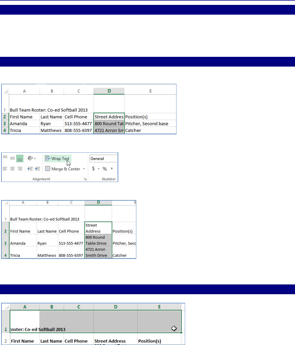
WRAP TEXT IN CELLS

1. Select the cells you wish to wrap.

2. Select the WRAP TEXT command on the HOME tab.

3. The text in the selected cells will be wrapped.

4. Click the Wrap Text command again to unwrap the text.

MERGE CELLS USING THE MERGE & CENTER COMMAND

1. Select the cell range you want to merge together.

2. Select the MERGE & CENTER command on the HOME tab.

3. The selected cells will be merged and the text will be centered.

Office of Information Technology Introduction to Microsoft Excel 2016

FORMATTING A WORKSHEET

Formatting changes the way that numbers and text are displayed in the worksheet, not their actual

value.

TEXT ALIGNMENT

By default, any text entered into your worksheet will be aligned to the bottom-left of a cell. Any

numbers will be aligned to the bottom-right of a cell. Changing the alignment of your cell content allows

you to choose how the content is displayed in any cell, which can make your cell content easier to read.

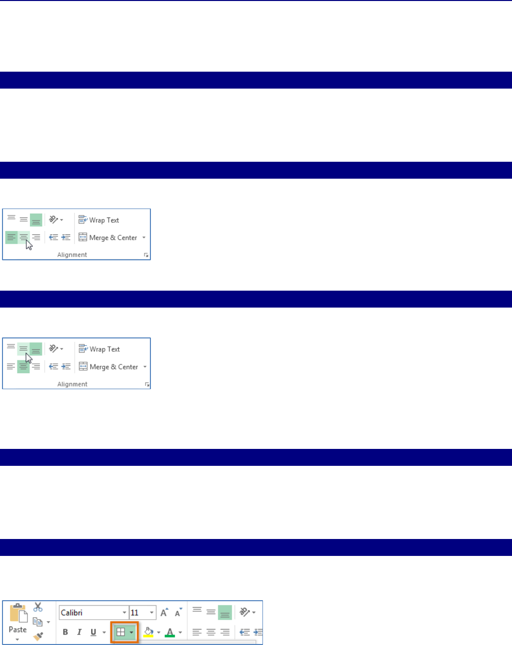
CHANGE HORIZONTAL TEXT ALIGNMENT

1. Select the cell(s) you wish to modify.

2. Select one of the three HORIZONTAL ALIGNMENT commands on the HOME tab.

3. The text will realign.

CHANGE VERTICAL TEXT ALIGNMENT

1. Select the cell(s) you wish to modify.

2. Select one of the three VERTICAL ALIGNMENT commands on the HOME tab.

3. The text will realign.

4. You can apply both vertical and horizontal alignment settings to any cell.

CELL BORDERS AND FILL COLORS

Cell borders and fill colors allow you to create clear and defined boundaries for different sections of

your worksheet. In our examples below, we'll add cell borders and fill color to our header cells to help

distinguish them from the rest of the worksheet.

ADD A BORDER

1. Select the cell(s) you wish to modify.

2. Click the drop-down arrow next to the BORDERS command on the HOME tab.

3. Select the border style you want to use.

4. The selected border style will appear.

5. You can draw borders and change the line style and color of borders with the DRAW

BORDERS tools at the bottom of the BORDERS drop-down menu.

Office of Information Technology Introduction to Microsoft Excel 2016

ADD A FILL COLOR

1. Select the cell(s) you wish to modify.

2. Click the drop-down arrow next to the FILL COLOR command on the HOME tab.

3. Select the fill color you want to use. A live preview of the new fill color will appear as you hover

the mouse over different options.

4. The selected fill color will appear in the selected cells.

FORMAT TEXT AND NUMBERS

One of the most powerful tools in Excel is the ability to apply specific formatting for text and numbers.

Instead of displaying all cell content in exactly the same way, you can use formatting to change the

appearance of dates, times, decimals, percentages (%), currency ($), and much more.

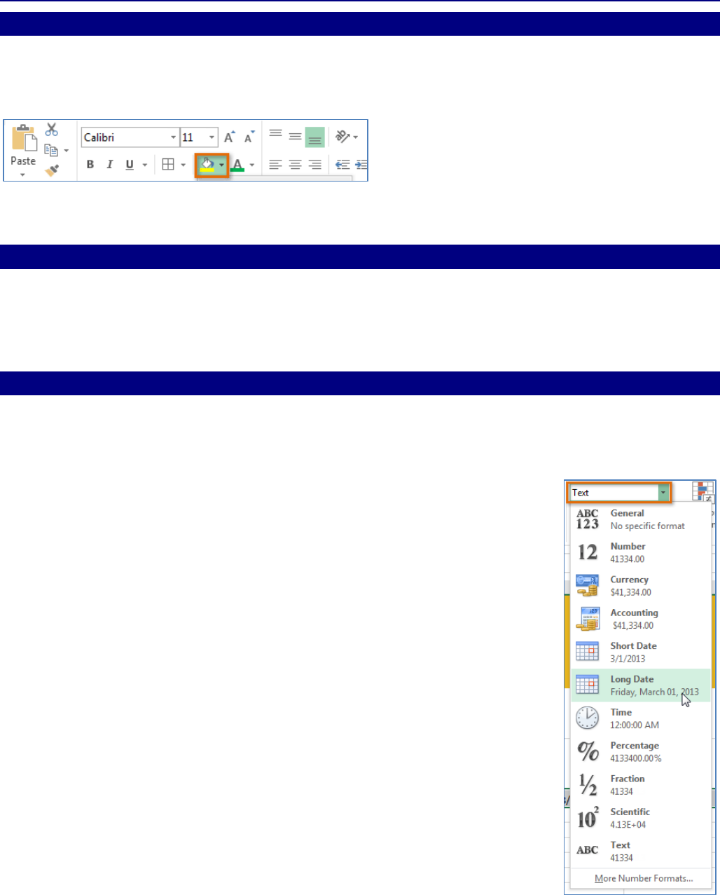
APPLY NUMBER FORMATTING

In our example, we will change the number format for several cells to modify the way dates are

displayed.

1. Select the cells(s) you wish to modify.

2. Click the drop-down arrow next to the NUMBER FORMAT command on the HOME tab.

3. Select the desired formatting option.

4. The selected cells will change to the new formatting style. For some

number formats, you can then use the Increase Decimal and Decrease

Decimal commands (below the NUMBER FORMAT command) to change

the number of decimal places that are displayed.

Office of Information Technology Introduction to Microsoft Excel 2016

WORKING WITH DATA – FREEZE PANES

FREEZE ROWS

You may want to see certain rows or columns all the time in your worksheet, especially header cells.

By freezing rows or columns in place, you'll be able to scroll through your content while continuing to

view the frozen cells.

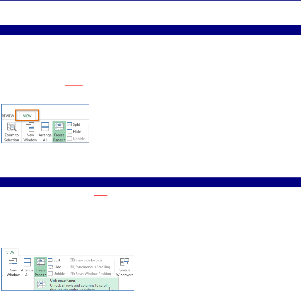
1. Select the row below the row(s) you wish to freeze.

2. Click the VIEW tab on the RIBBON.

3. Select the FREEZE PANES command and then choose FREEZE PANES from the drop-down menu.

4. The rows will be frozen in place, as indicated by the gray line. You can scroll down the worksheet

while continuing to view the frozen rows at the top.

FREEZE COLUMNS

1. Select the column to the right of the column(s) you wish to freeze.

2. Click the VIEW tab on the RIBBON.

3. Select the FREEZE PANES command and then choose FREEZE PANES from the drop-down menu.

4. The column will be frozen in place, as indicated by the gray line. You can scroll across the

worksheet while continuing to view the frozen column on the left.

5. To unfreeze rows or columns, click the FREEZE PANES command and then select UNFREEZE

PANES from the drop-down menu.

6. If you only need to freeze the top row (row 1) or first column (column A) in the worksheet, you

can simply select FREEZE TOP ROW or FREEZE FIRST COLUMN from the drop-down menu.

Office of Information Technology Introduction to Microsoft Excel 2016

USING FORMULAS AND FUNCTIONS

Formulas consist of the addresses of the cells containing the values and the appropriate mathematical

operators. Formulas begin with an equal sign (=), because they contain cell addresses. This prevents

Excel from interpreting the formula as text, since cell addresses begin with letters. For example, to add

the numbers in cells A1 and A2, you would type the formula: =A1+A2.

You enter the formula in the cell where you want the result to appear. Because formulas use cell

addresses, they automatically recalculate when the value of a cell used in a formula changes. When a

cell containing a formula is selected, the actual formula appears in the formula bar. The calculated

results of the formula appear in the cell.

+ for addition

- for subtraction

* for multiplication

/ for division

^ for exponents

A Function is a formula or action that is built into Excel. For example, rather than use the plus sign (+) to

add cells A1 through A5, use the SUM function: =SUM(A1:A5)

ORDER OF OPERATIONS

When you are examining or creating formulas, you should keep in mind that there is a specific sequence

that Excel follows when it performs calculations. This is the order of operations:

1. Parentheses: computations enclosed in parentheses are first priority.

2. Exponents: computations involving exponents are performed next.

3. Multiplication and division: these operations are performed next in the order in which they are

encountered (from left to right).

4. Addition and subtraction: these operations are performed last. They are also performed in the

order in which they are encountered (from left to right).

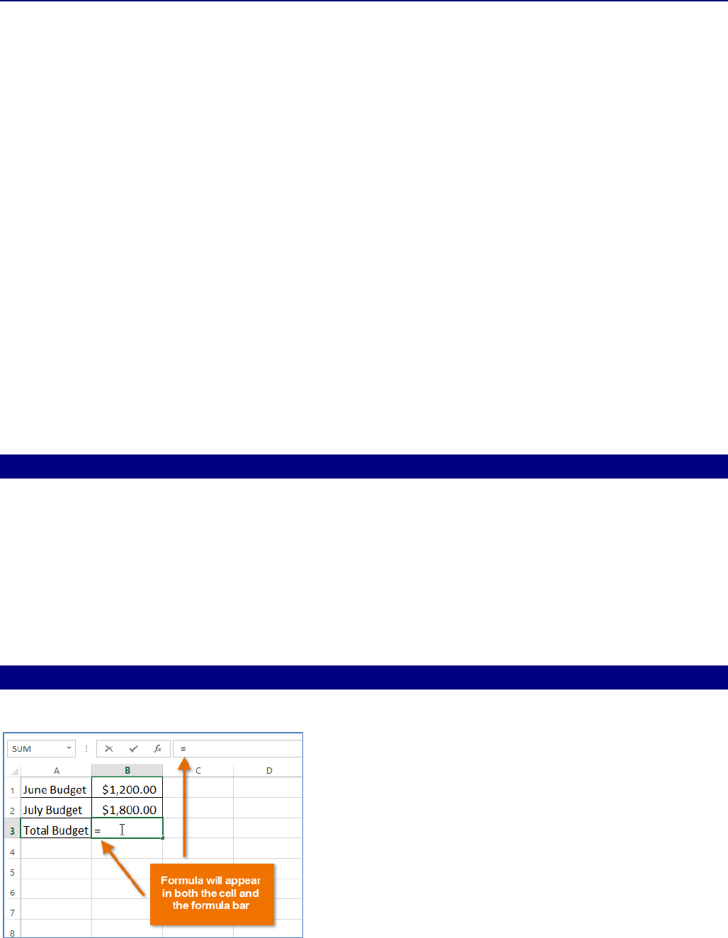
CREATE A FORMULA

1. Select the cell that will contain the formula.

2. Type the equal sign (=). Notice how it appears in both the cell and the formula bar.

Office of Information Technology Introduction to Microsoft Excel 2016

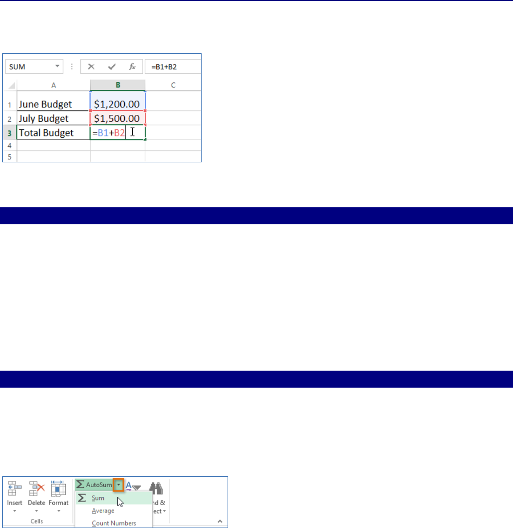
3. Type the cell address of the cell that you wish to reference first in the formula.

4. Type the mathematical operator you wish to use.

5. Type the cell address of the cell that you wish to reference second in the formula.

6. Press ENTER on your keyboard. The formula will be calculated and the value will be displayed in

the cell.

COMMON FUNCTIONS

Excel has a wide variety of functions available. Here are some of the most common functions you'll use:

 SUM: This function adds all the values of the cells in the argument.

 AVERAGE: This function determines the average of the values included in the argument. It

calculates the sum of the cells and then divides that value by the number of cells in the

argument.

 COUNT: This function counts the number of cells with numerical data in the argument. This

function is useful for quickly counting items in a cell range.

 MAX: This function determines the highest cell value included in the argument.

 MIN: This function determines the lowest cell value included in the argument.

CREATE A FUNCTION USING THE AUTOSUM COMMAND

The AUTOSUM command allows you to automatically insert the most common functions into your

formula, including SUM, AVERAGE, COUNT, MIN, and MAX. Select the cell that will contain the function.

In our example, we'll select cell D12.

1. In the EDITING group on the HOME tab, locate and select the arrow next to

the AUTOSUM command and then choose the desired function from the drop-down menu.

2. The selected function will appear in the cell. If logically placed, the AUTOSUM command

will automatically select a cell range for the argument.

 You can also manually enter the desired cell range into the argument.

3. Press ENTER on your keyboard. The function will be calculated and the result will appear in the

cell.

4. The AUTOSUM command can also be accessed from the FORMULAS tab on the RIBBON.

Office of Information Technology Introduction to Microsoft Excel 2016

RELATIVE AND ABSOLUTE CELL REFERENCES

There are two types of cell references: relative and absolute. Relative and absolute references behave

differently when copied and filled to other cells. Relative references change when a formula is copied to

another cell. Absolute references, on the other hand, remain constant, no matter where they are

copied.

RELATIVE REFERENCES

By default, all cell references are relative references. When copied across multiple cells, they change

based on the relative position of rows and columns. For example, if you copy the formula =A1+B1 from

row 1 to row 2, the formula will become =A2+B2. Relative references are especially convenient

whenever you need to repeat the same calculation across multiple rows or columns.

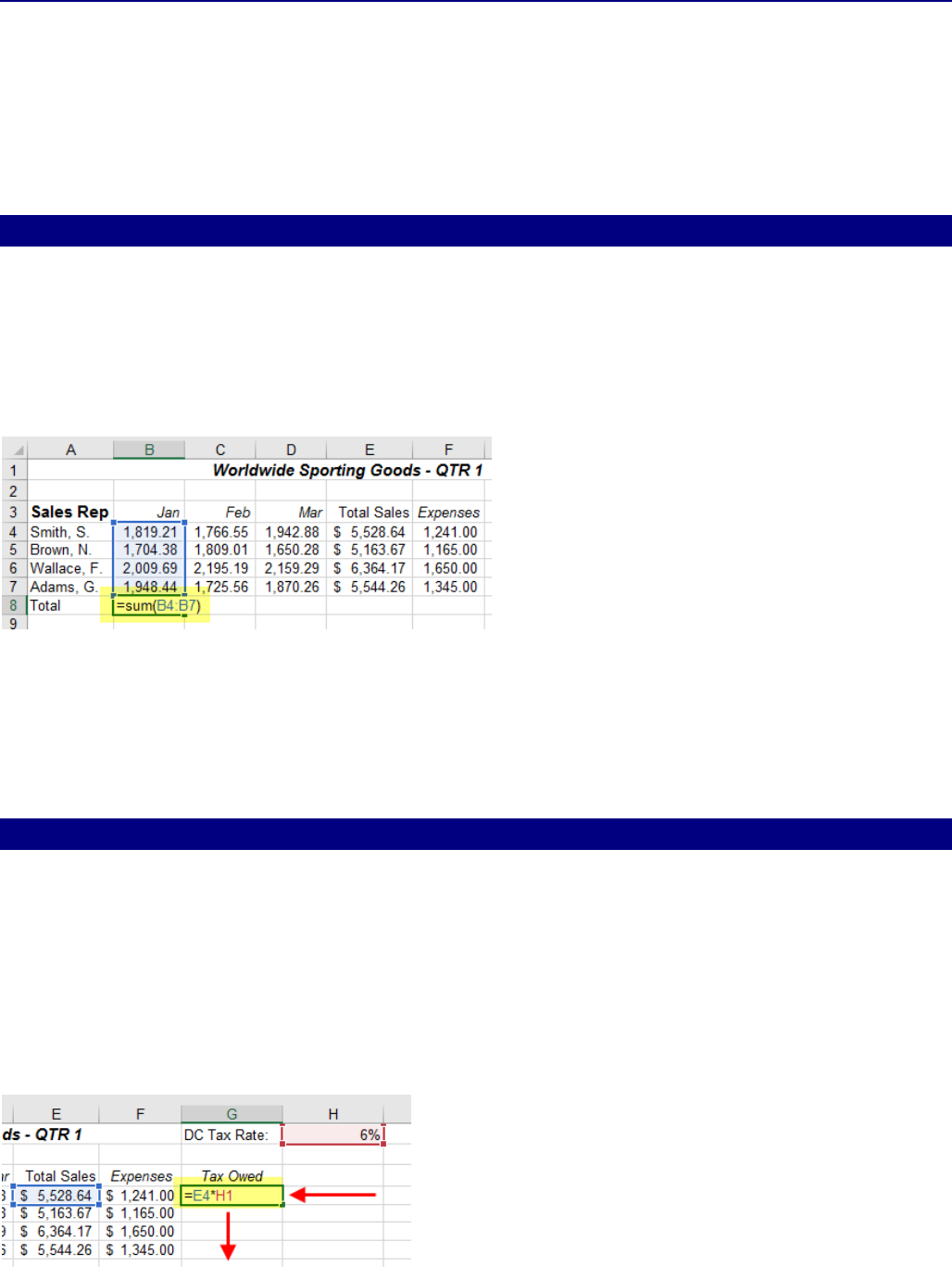
1. Enter the formula to calculate the desired value. In our example, we'll type =SUM(B4:B7).

2. Locate the fill handle in the bottom-right corner of B8.

3. Click, hold, and drag the fill handle over the cells you want to fill. In our example, we'll select cells

C8:F8.

4. Release the mouse. The formula will be copied to the selected cells with relative references, and

the values will be calculated in each cell.

ABSOLUTE REFERENCES

There may be times when you do not want a cell reference to change when filling cells. Unlike relative

references, absolute references do not change when copied or filled. You can use an absolute reference

to keep a row and/or column constant. An absolute reference is designated in a formula by the addition

of a dollar sign ($). It can precede the column reference, the row reference, or both.

Enter the formula to calculate the tax owed on sales for Qtr 1 for the 1

salesperson. Then, copy the

formula for each of the remaining 3 salespersons.

The dollar signs were omitted in the example. This

caused Excel to interpret it as a relative reference,

producing an incorrect result when copied to other cells.

Be sure to include the dollar sign ($) whenever you're

making an absolute reference across multiple cells.

Office of Information Technology Introduction to Microsoft Excel 2016

PASTE SPECIAL

When you copy the contents of a cell or a range of cells to the Windows Clipboard, any formatting that

has been applied is copied as well as the cell contents. When you subsequently paste the contents of the

Clipboard to a new location, an exact copy of both the contents and the formatting is pasted.

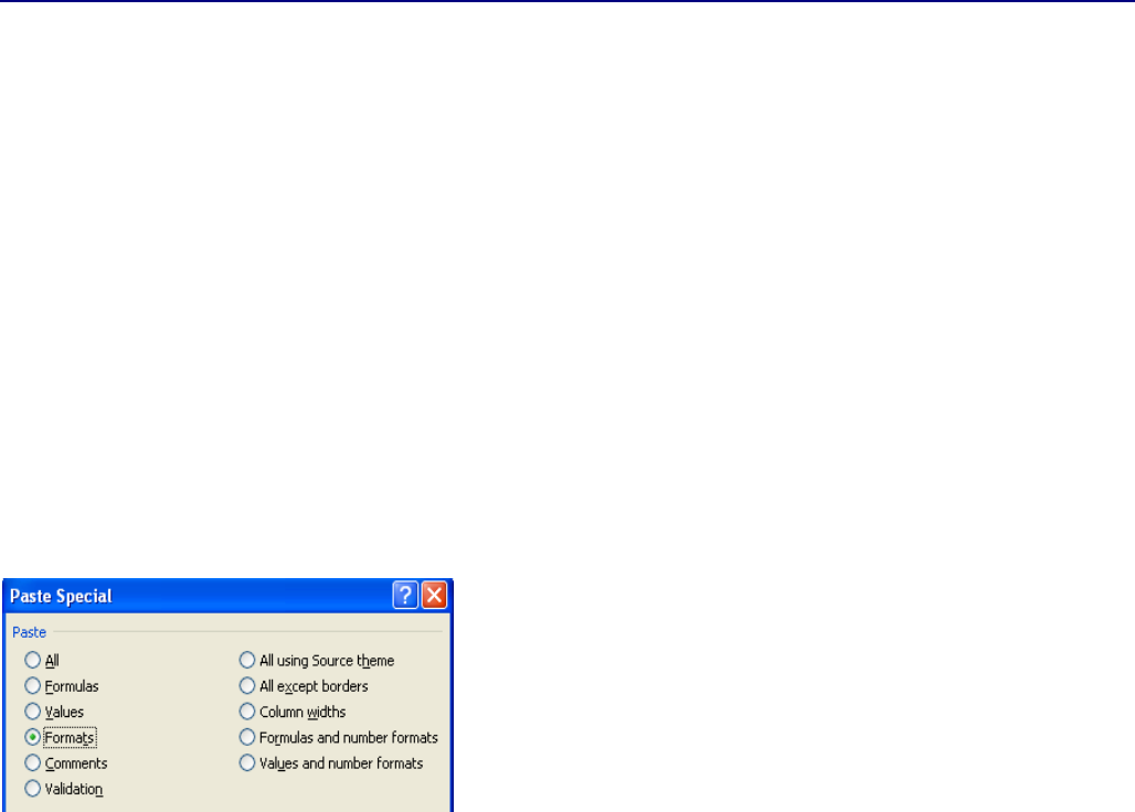
There may be times when you want to paste only certain aspects of the copied cells (such as formulas,

values, or formats). For example, you may want to copy the formats of an entire worksheet to another

worksheet but not the data or values. The Paste Special command allows you to specify what you want

to paste into the new location. You can paste all cell attributes or only selected ones.

COPY FORMATS

1. Select the QTR 3 worksheet and apply formatting to the column headings.

2. Select those cells and click the COPY button in the HOME tab.

3. Select the QTR 4 tab and select the column heading cells.

4. Click the dropdown arrow on the PASTE button on the HOME tab.

5. Select PASTE SPECIAL and choose FORMATS. Click OK.

COPY VALUES

6. To copy the results of a formula, but not the formula itself, select a cell that contains a

formula. Then, click the COPY button.

7. Select a blank cell in the same worksheet or on another worksheet.

8. Click the dropdown arrow on the PASTE button on the HOME tab.

9. Select PASTE SPECIAL and choose VALUES. Click OK.

COPY FORMULAS

10. To copy a formula so the formula can be used on another worksheet, select a cell that

contains a formula. Then, click the COPY button.

11. Click the dropdown arrow on the PASTE button on the HOME tab.

12. Select PASTE SPECIAL and choose FORMULAS. Click OK.

Office of Information Technology Introduction to Microsoft Excel 2016

RANGE NAMES

Advantages to using Range Names instead of cell addresses include:

 Names reduce the chance of error in formulas. It’s easy to recognize if EXPENSES is typed

incorrectly. If a cell address is typed incorrectly, it is harder to detect.

 Names adapt to changes within a range (for example, when rows and columns are added to or

removed from the range).

 Names are easy to recognize and maintain in formulas. For example, the formula =TOTALSALES -

EXPENSES is easier to understand than the formula =E3 - F3.

 You can easily go to a named cell or range using the Name box (or F5).

 Names created in one worksheet are available to all other worksheets in the workbook.

 Names are absolute. If you use a range name in a formula, the formula always refers to that

range even if you copy or move the formula.

ASSIGN A NAME TO A RANGE USING THE NAME BOX

You can use names instead of cell There are some specific rules for assigning names to ranges:There are

some specific rules for assigning names to ranges:

o Names must start with a letter or an underscore character. The remainder of the name can

contain any character except a space or a hyphen. Names are not case-sensitive.

o Names can be up to 255 characters long; however, you should keep them short to make them

easy to use and to conserve space in formulas.

o You should not use names that resemble cell references (such as A1).

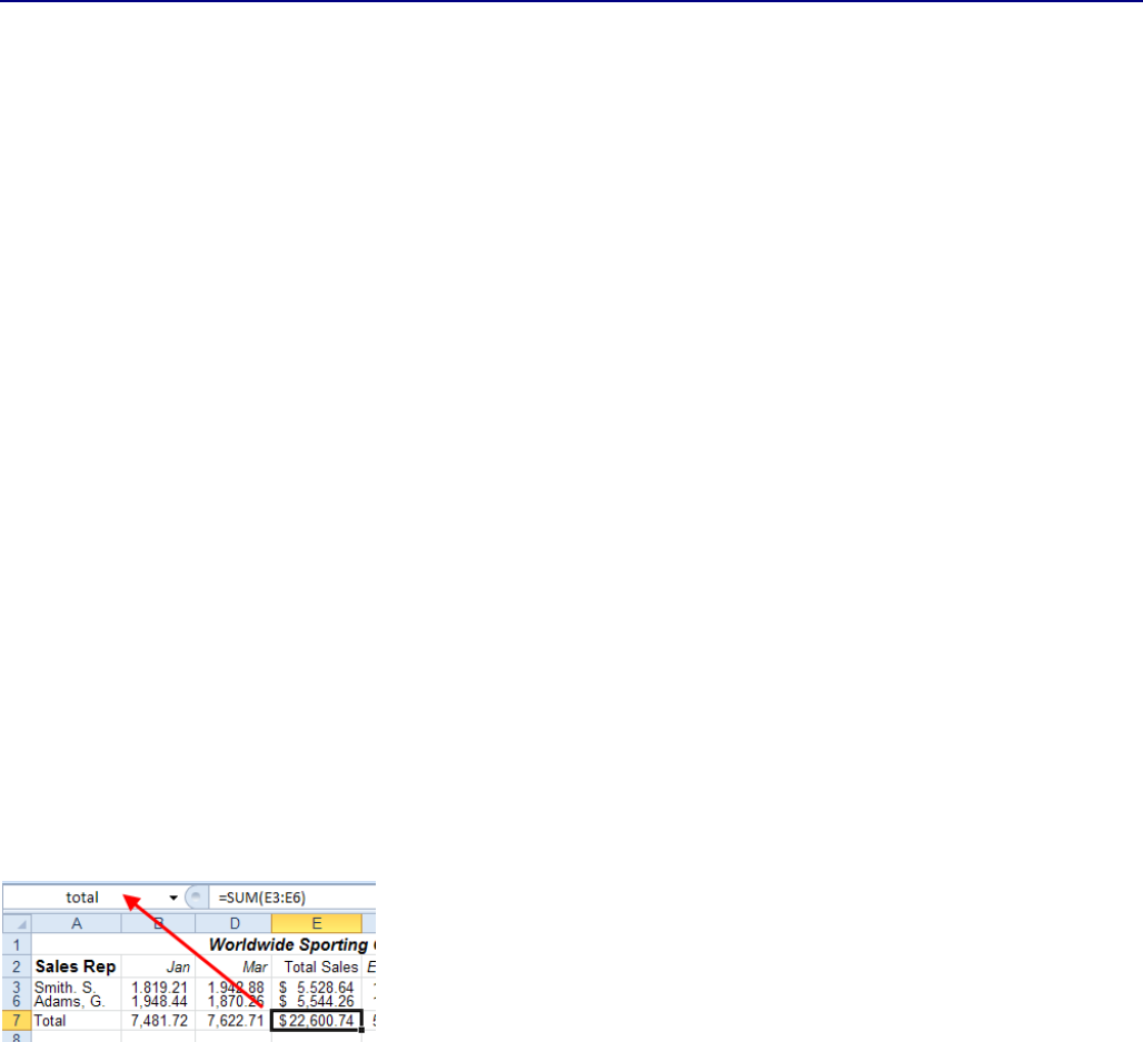
13. In the spreadsheet ADDSAL1, click on a cell that contains a formula, such as Total Sales.

14. Click in the NAME box, type total and press ENTER.

GO TO A NAMED RANGE

15. Open the ADDSAL1 workbook in the Excel Advanced Samples folder.

16. Press the GOTO key, F5.

17. Either type ‘total’ or double-click ‘total’ if it appears in the box.

18. The cursor will now be positioned on the cell that you named ‘total’.

Office of Information Technology Introduction to Microsoft Excel 2016

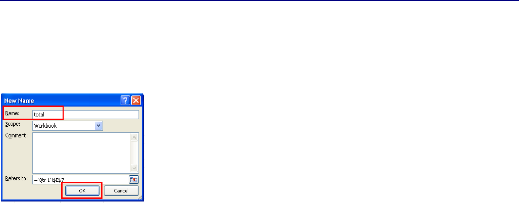
ASSIGN A NAME TO A RANGE USING THE NAME MANAGER

19. In the worksheet, click on a cell that contains a total formul.

20. Click NAME MANAGER in DEFINED NAMES on the FORMULAS TAB.

21. Click NEW.

22. Type total in the NAME field, click OK, then, click CLOSE.

USE A NAMED RANGE IN A FORMULA

23. IN A BLANK CELL IN THE SPREADSHEET, ENTER =E4/TOTAL in a blank cell and press ENTER.

24. The current value of ‘total’ will be used in the formula.

DELETE A RANGE NAME

Deleting a range name permanently removes it from the workbook. If you accidentally delete a range

name that is still referred to in a formula, the formula can no longer calculate correctly, and the error

message #NAME? appears in the cell instead of the result of the formula.

25. Click the NAME MANAGER button. The NAME MANAGER window will open.

26. Select total.

27. Click the DELETE button, click OK, then, click CLOSE.

Office of Information Technology Introduction to Microsoft Excel 2016

WORKING WITH DATA – SORT AND FILTER

Excel 2016 contains enhanced data filtering features that allow you to sort and filter data and easily

remove duplicate data entries.

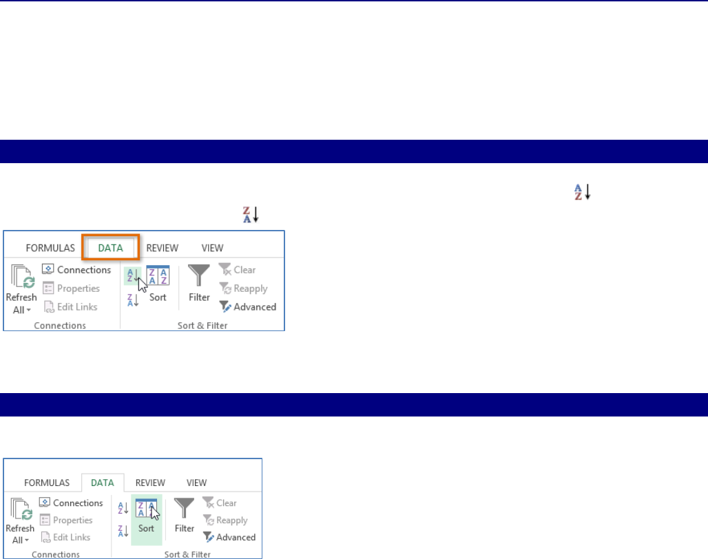
SORT A SHEET

1. Select a cell in the column you wish to sort by.

2. Select the DATA tab on the RIBBON and then click the ASCENDING command to Sort A to Z, or

the DESCENDING command to Sort Z to A.

3. The worksheet will be sorted by the selected column.

SORT A RANGE

1. Select the cell range you wish to sort.

2. Select the DATA tab on the RIBBON and then click the SORT command.

3. The SORT dialog box will appear. Choose the column you wish to sort by.

4. Decide the Sorting Order.

5. Click OK.

6. The cell range will be sorted by the selected column.

4. If your data isn't sorting properly, double-check your cell values to make sure they are entered

into the worksheet correctly. Even a small typo could cause problems when sorting a large

worksheet.

Office of Information Technology Introduction to Microsoft Excel 2016

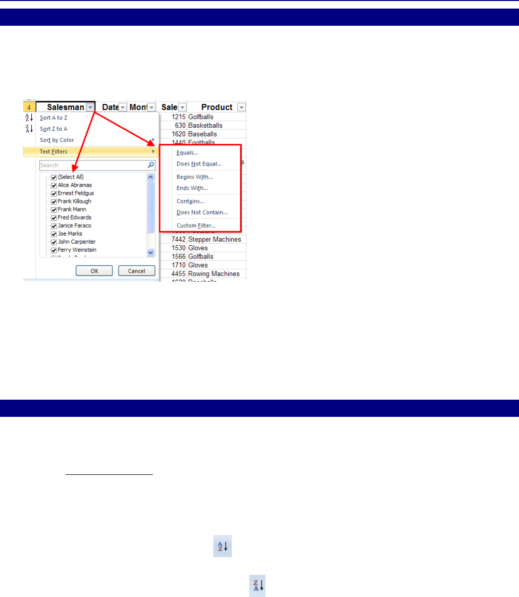
AUTOFILTER

The AutoFilter option allows you to hide records in a list except those that meet certain criteria. The

AutoFilter command places a drop-down menu at the top of each column in the list. To display a filtered

group of records from the menu, select the criteria from the list.

28. Open the file PIVOT1.XLSX.

29. Select the cell containing the column heading Salesman.

30. On the DATA tab, click the FILTER button in the SORT & FILTER group.

31. Click the arrow next to SALESMAN. A Sort menu will appear. Deselect SELECT ALL and select

ALICE ABRAMAS. The sorted data will appear in your spreadsheet.

32. To clear the sort, click the CLEAR button in the SORT & FILTER group.

USING FILTER TO SORT

The Sort Ascending and Sort Descending buttons allow you to sort individual rows in a column, or to

sort rows in a worksheet based on the values in one column only. The SORT button gives you the ability

to sort using additional criteria.

1. If using the file PIVOT.XLSX, select cells A4: I29.

2. You can also just select a column heading as long as there are no blank rows between the

column headings and the data.

3. Click the SORT ASCENDING button, . Notice that the data has been sorted alphabetically by

the first column.

4. Then, click the SORT DESCENDING button, . Notice the data in the first column has been

sorted in reverse order.

Office of Information Technology Introduction to Microsoft Excel 2016

PRINTING THE WORKSHEET

WORK WITH HEADERS AND FOOTERS

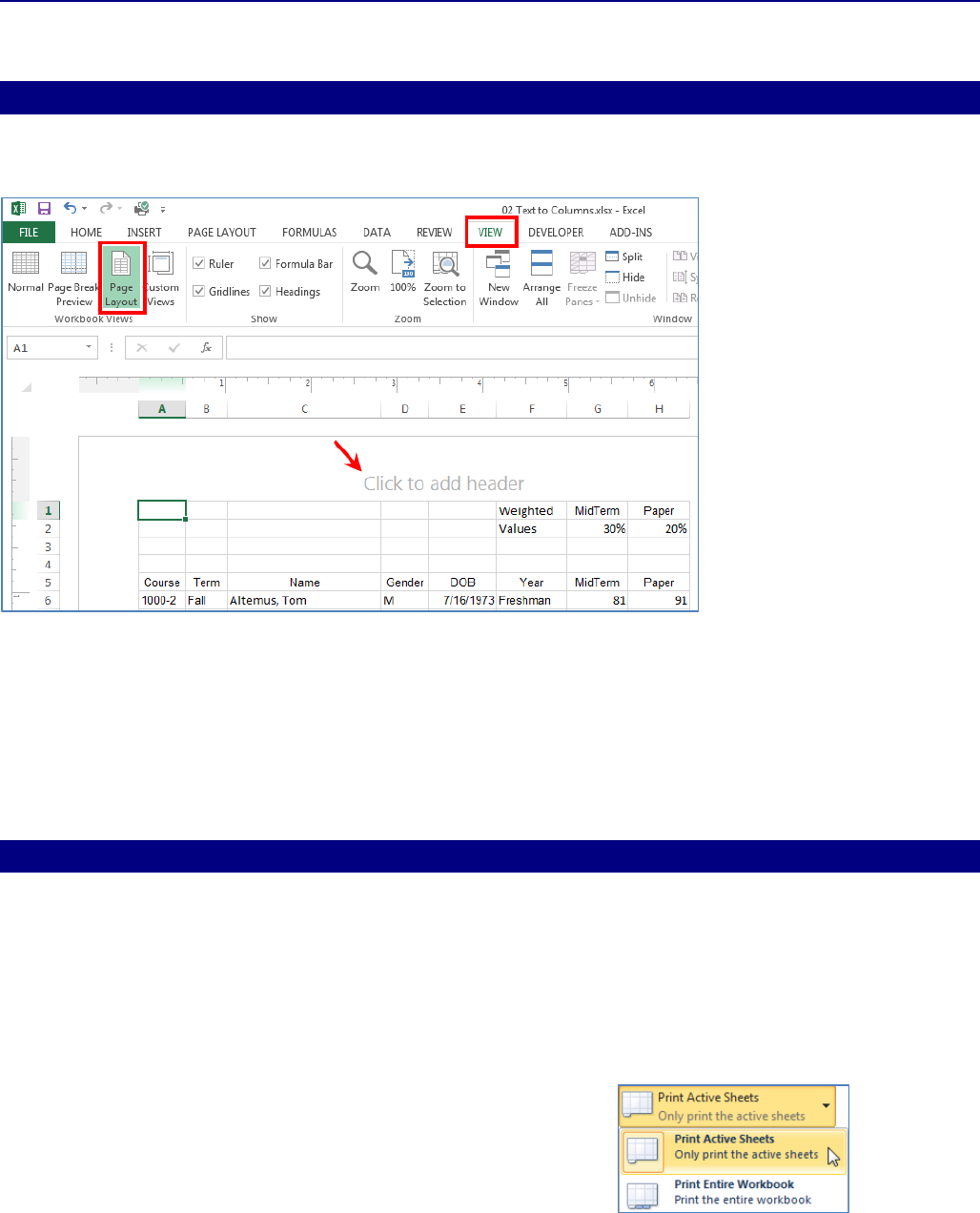
1. In the View tab, click PAGE LAYOUT in the WORKBOOK VIEWS group.

2. Click the CLICK TO ADD HEADER link and type your header text directly into the box.

3. Press the [ENTER] key when you are done. The header will display.

4. Note that when you click a header or footer section, the DESIGN contextual tab will display in the

ribbon. This tab contains additional formatting tools.

5. To create a footer, click the GO TO FOOTER link on the NAVIGATION group of the DESIGN tab and

type the footer text.

6. Click off the header or footer to deselect this option.

PRINT THE ACTIVE WORKSHEET

If you have multiple worksheets in your workbook, you will need to decide if you want to print the whole

workbook or specific worksheets. Excel gives you the option to PRINT ACTIVE SHEETS. A worksheet is

considered active if it is selected.

1. Select the worksheets you want to print. To print multiple worksheets, click on the first worksheet,

hold down the CTRL key, then click the other worksheets you want to select.

2. Click the FILE tab.

3. Select PRINT to access the Print pane.

4. Select PRINT ACTIVE SHEETS from the print range drop- down

menu.

5. Click the PRINT button.

Office of Information Technology Introduction to Microsoft Excel 2016

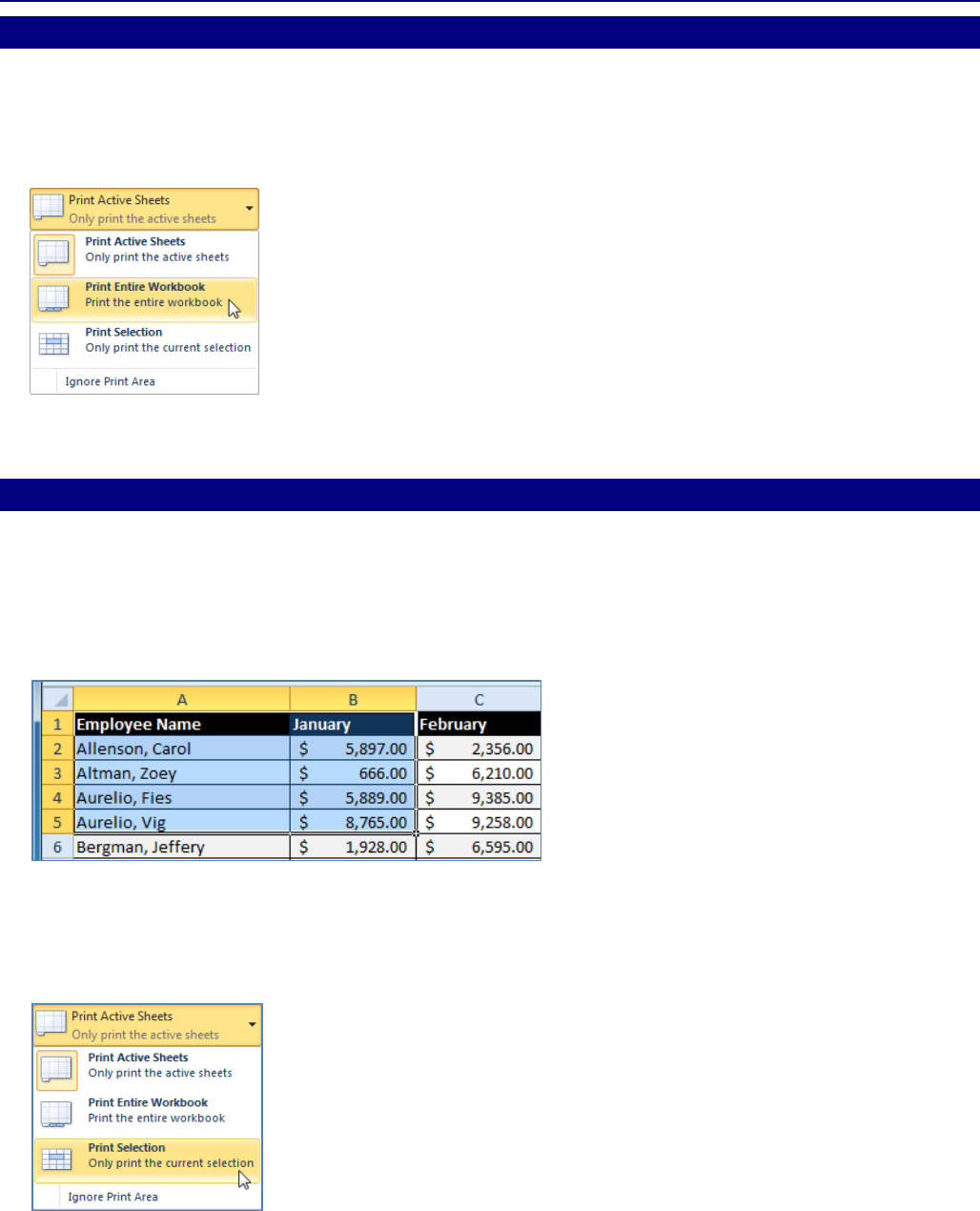
PRINT THE ENTIRE WORKBOOK

1. Click the FILE tab.

2. Select PRINT to access the Print pane.

3. Select PRINT ENTIRE WORKBOOK from the print range drop-down menu.

4. Click the PRINT button.

PRINT A SELECTION OR SET THE PRINT AREA

Printing a selection (sometimes called setting the print area) lets you choose which cells to print, as

opposed to the entire worksheet.

1. Select the cells that you want to print.

2. Click the FILE tab.

3. Select PRINT to access the Print pane.

4. Select PRINT SELECTION from the print range drop-down menu.

5. You can see what your selection will look like on the page in PRINT PREVIEW.

6. Click the PRINT button.

Office of Information Technology Introduction to Microsoft Excel 2016

SAVING A FILE

When you save a workbook for the first time, Excel opens the Save As dialog box in which you enter the

desired file name and location. Excel 2016 automatically assigns the .xlsx extension when you are saving

a file.

As in previous versions of Excel, you can save files locally to your computer. But unlike older versions,

Excel 2016 also lets you save a workbook to the cloud using SkyDrive. You can also

export and share workbooks with others directly from Excel.

Once a workbook has been saved to disk, its file name appears in the application title bar. Excel updates

the existing file each time you subsequently save the workbook. You can also select the SAVE command

from the FILE menu to save a workbook.

Excel offers two ways to save a file: Save and Save As. These options work in similar ways, with a few

important differences:

 Save: When you create or edit a workbook, you'll use the Save command to save your changes.

You'll use this command most of the time. When you save a file, you'll only need to choose a file

name and location the first time. After that, you can just click the Save command to save it with

the same name and location.

 Save As: You'll use this command to create a copy of a workbook while keeping the original.

When you use Save As, you'll need to choose a different name and/or location for the copied

version.

Office of Information Technology Introduction to Microsoft Excel 2016

SAVE A WORKBOOK

1. Locate and select the SAVE command on the Quick Access Toolbar.

2. If you're saving the file for the first time, the SAVE AS pane will appear in Backstage view.

3. You'll then need to choose where to save the file and give it a file name. To save the workbook to

your computer, select COMPUTER and then click BROWSE.

4. The SAVE AS dialog box will appear. Select the location where you wish to save the workbook.

5. Enter a file name for the workbook and click SAVE.

6. The workbook will be saved. You can click the SAVE command again to save your changes as you

modify the workbook.

7. You can also access the SAVE command by pressing CTRL+S on your keyboard.

USE SAVE AS TO MAKE A COPY

If you want to save a different version of a workbook while keeping the original, you can create a copy.

For example, if you have a file named "Sales Data" you could save it as "Sales Data 2" so that you'll be

able to edit the new file and still refer back to the original version.

To do this, you'll click the SAVE AS command in Backstage View. Just like when saving a file for the first

time, you'll need to choose where to save the file and give it a new file name.

EXPORT A WORKBOOK AS A PDF FILE

A PDF file will make it possible for recipients to view, but not edit, the content of your workbook.

1. Click the FILE tab to access Backstage view.

2. Click EXPORT and then select Create PDF/XPS.

3. The Save As dialog box will appear. Select the location where you wish to export the workbook,

enter a file name, then click PUBLISH.

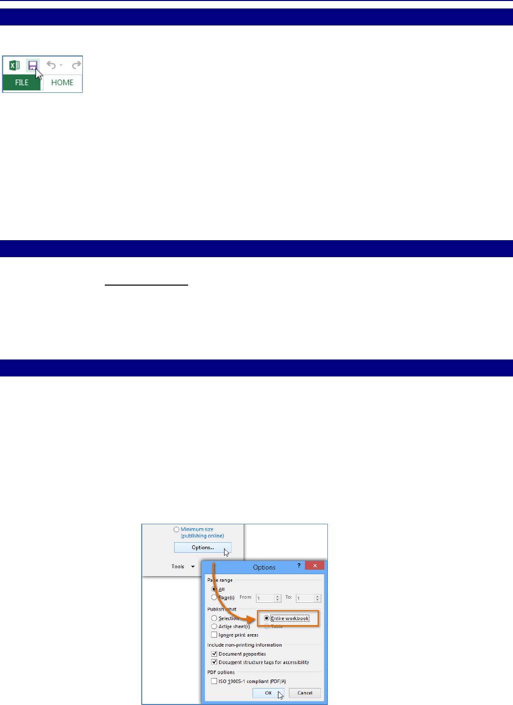
 By default, Excel will only export the active worksheet. If you have multiple worksheets

and want to save all of them in the same PDF file, click OPTIONS in the Save as dialog box.

The OPTIONS dialog box will appear. Select ENTIRE WORKBOOK and then click OK.